Supervised Learning
In supervised learning, we take some data and predict an output in a pre-defined structure. There are two categories:
- Regression: When a function is given some input variables, what is the continuous output?
- i.e. for \(y = f(x)\), what is \(y\) for various \(x\)?
- Examples: Linear Regression, Logistic Regression
- Classification: When a function is given some input variables, which variables map to a distinct category?
- i.e. If \(f(x) = ax + bx+ c\) shows us the results of the cancer scan, and \(a\) represents the amount of mercury consumption in a human, does \(a\) map to 'benign' cancer or 'malignant' cancer?
- Examples: Image Classification
Models and Training
Models are systems that maps inputs (features) to outputs (labels). Features are also known as \(x\), and labels are known as \(y\). Labels are known in supervised learning and semi-supervised learning algorithms.
- Models learn relationships between features and labels
- i.e. prices (label) are higher for houses with greater sq. ft (feature)
- Models are used for supervised learning (i.e. regression, neural networks)
- Models learn from training data to become trained models
- Trained models are evaluated with testing data
Fitting
Models are fitted with training data. Fitting is synonymous with learning, but it is a more mathematical term used to represent fitting values \(m\) and \(b\) inside a hypothetical model that can be generally represented as the function \(y = mx + b\).
Underfitting

Underfitting occurs when the model doesn't accurately represent the relation between the feature input and the label output of the training data. For example, a linear function to represent data that clearly has a zig-zag trend as \(x\) grows larger is not the best fit for this data - a higher order polynomial function (such as a quadratic equation) would produce a more accurate result. The linear function in this case gives high bias, due to its bias for linearity contrary to the actual data's polynomial curve.
Overfitting

Overfitting occurs when the model is trained too strictly based on the data. This is the opposite of underfitting; for example, a cubic function to represent data that has a quadratic trend. This results in incredibly good predictions on training data, but for test data or unseen data, it will perform quite badly due to the high variance levels of the trained model. The model becomes too reliant on the pattern of the training data set, causing test sets to suffer poorly for predictions.
Training, Validation, and Test Datasets
The best way to view these three datasets:
          Entire Dataset
          /            \
      Training        Test
     /        \
Reduced    Validation
Training Dataset
- This is the dataset that is used to simply train the model
- Can be further split into a reduced Training set and a Validation set.
Test Dataset
- This is the dataset that we test against with our trained model. It is split off from the entire dataset and is separate from the training dataset.
- The goal is to have accurate predictions with our test data, based on our trained model
Reduced Dataset
- In the case that we want to use validation datasets, we split the training dataset into a reduced training dataset, which is what we will use to train our model. The other portion is used for the validation dataset.
Validation Dataset
- Used to reduce overfitting as the model is being trained. If the training dataset has high accuracy but the validation dataset has low accuracy, then the model should re-tune its hyperparameters.
- In general, a key distinction between test datasets and validation datasets is that with test datasets, you may not have the outputs. With validation datasets, you have the outputs. This means that you can calculate the accuracy of trained datasets and validation datasets, which means you can keep refining your model to improve its accuracy.
- Test datasets can therefore be seen as a final validation dataset which is used to measure the accuracy of your deployed model. (examples: Kaggle datasets)
- You can split up the training dataset into a validation set and a reduced training set - this gives you the outputs/labels for both datasets. With Keras, you can define the
validation_splitparameter in the.fitfunction to implicitly create a validation set.
Linear Regression
In linear regression, you have some data (features) that will produce an output. There are two variations; SLR (Simple Linear Regression) and Multivariate Linear Regression.
Cost Function
The cost function will output the ratio of accuracy between the predicted output and the actual output. Think of this as an auditing function.
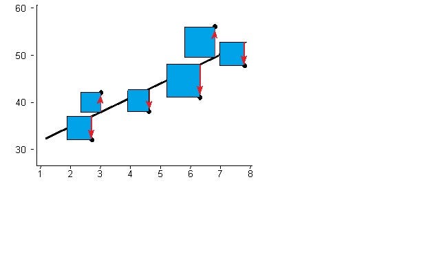
MSE (Mean Squared Error) is a popular cost function.
def cost_function(radio, sales, weight, bias):
    companies = len(radio)
    total_error = 0.0
    for i in range(companies):
        total_error += (sales[i] - (weight*radio[i] + bias))**2
    return total_error / companies
Takeaway: Smaller the better.
Gradient Descent
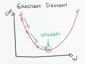
Gradient Descent is one way to optimize the parameters (feature weights) in multivariate linear regression. One use case in particular is to lower the MSE cost function (above), which is always a good thing.
The basic idea is that it is used to minimize some function by iteratively moving in the direction of the steepest descent.
It uses calculus and derivatives to find a negative gradient, with the output being coordinates for a new point. These new coordinates then get fed to the same function as parameters, finding an even lower negative gradient. Each iteration is known as the learning rate. Essentially, it will reach a point where it doesn't really go much lower, and arrives at the local minimum.

Takeaway: This is a super fast way to optimize weights, and Scikit also offers a library for this (see SGD).
OLS (Ordinary Least Squares)
Ordinary Least Squares is a function that is simpler (mathematically) and it is popular for its use in sklearn.linear_model.LinearRegression. OLS and Gradient Descent both gets the job done for optimizing weights, but OLS is slower when there are huge datasets for multivariate regressions.
 The goal is fairly simple - minimize the sum of the squared errors (closer to the slope line, the better.)
Takeaway: Use OLS for simple problems but if the dataset is huge, use Gradient Descent instead since it is computationally much faster.
Normalization
Normalization just means to make all of our input data within the "normal" range respective to each other. If one feature had a range of 1000 - 5000, and another feature had a range of 0-5, then clearly the first feature will have a very undistributed weight and will skew the output greatly.
Note: Normalization doesn't really make sense for SLR (Simple Linear Regression) since you are only dealing with one feature. It makes sense for problems with multiple features, and numeric features at that.
One Hot Encoding
One Hot Encoding is a technique to convert categorical data into numerical data in such a way that your model can better interpret the meaning of the data. This is useful in scenarios where the categorical data doesn't have a lot of meaning when converted to numbers. For example, assigning colors red = 1, blue = 2, and green = 3 doesn't really have much meaning across varying applications.
With One Hot Encoding, you basically turn your categorical data into binary data that is classified by state (1 for yes, 0 for no). Note that you will have more columns - one for each classification of the data.
red | blue | green
 1     0     0
 0     1     0
 0     0     1
def normalize(features):
    **
    features     -   (200, 3)
    features.T   -   (3, 200)

    We transpose the input matrix, swapping
    cols and rows to make vector math easier
    **

    for feature in features.T:
        fmean = np.mean(feature)
        frange = np.amax(feature) - np.amin(feature)

        #Vector Subtraction
        feature -= fmean

        #Vector Division
        feature /= frange

    return features
Prediction function / Hypothesis
The prediction function is simply the \(y = mx + b\) equation for Simple Linear Regression or \(y = ax1 + bx2 + cx_3 + ...\) for multivariate linear regression. It's basically the main crux algorithm for determining the predicted output.]
Heuristic
A heuristic is an estimation function and is normally a hand-coded function. For example, the A* algorithm uses heuristics for searching. At its core, it is a helper function.
In a ML context, it is not based on a model obtained by training on a data set, but typically embodies some common-sense expertise from domain experts. ML algorithms can use heuristics (based on definitive logic) to solve a problem more quickly.
Model Parameters
Parameters are configurations used to tune a model, which are estimated or derived from the data. These values are specific to the model, so parameters for one model may not be the best for another model.
- Weights in Neural Networks
- Coefficients used in Linear Regression
Model Hyperparameters
Hyperparameters are configurations used to tune the machine learning algorithm and are not derived from data. Instead, these values are, generally speaking, inputted manually and cannot be derived automatically. We often come up with hyperparameters through heuristics, assumptions or trial-and-error experiments.
- Learning rate for neural networks
- C and sigma values for SVM (Support Vector Machines)
- The k value in k-nearest neighbors
Neural Networks
A neural network involves neurons (or perceptrons), weights and layers.
At the most basic level, inside a neural network there is an input layer, an output layer, and hidden layers which are any layers between the input and output layers. The overall goal is to feed in some input features \(x\) (represented conceptually as neurons) into the input layer, multiply them with their corresponding weights \(w\), feed the results into any additional hidden layers (at this stage, we would be dealing with densely connected layers), until finally the weights at the last layer are summed and a bias is applied to find the output \(\hat{y}\).
Activation Functions
The activation function allows for the network to handle non-linearities in the input, which means we would be able to better predict complex functions. Note that the bias applied to the final stage of neural networks (mentioned above) is done by applying the activation function.

For example, to capture the input above, a simple linear function would not be able to do the job effectively - the blue outline capturing the plots above represents a non-linear function.
Some common activation functions:
- tan
- ReLU
- sigmoid
Cost Function
In neural networks, the concept of loss still exists, except that calculating the loss can be a bit more trickier when we have to apply back-propagation with a densely connected network.
Unsupervised Learning
Unsupervised learning is basically any kind of machine learning that has no structure (or labels) defined for your input data.
Techniques to cover
- Random Cut Forests
Reinforcement Learning
Reinforcement Learning is a type of machine learning where you receive data piece by piece which will either give you a "good" signal or "bad" signal, and over time your model will learn to discard the "bad" signals in order to reach the best outcome.